A classifier says an applicant has an 80% chance of repaying a loan. Another predicts that a transaction has a 95% probability of being fraudulent. Those percentages look precise, but do they correspond to observed frequencies? AI model calibration addresses the relationship between predicted probabilities and actual outcomes. A model can rank cases effectively while giving misleading confidence scores—a serious problem when those scores guide decisions.
Calibration is not a guarantee that each individual prediction will be right. It is a statistical property evaluated across sets of predictions. If a model assigns roughly 0.8 probability to many comparable events, approximately 80% should occur in a sufficiently representative sample for that group to be well calibrated. Understanding this distinction changes how teams select thresholds, estimate risk, and communicate uncertainty.
Why accuracy and calibration are different
Imagine two systems predicting whether packages will arrive late. Model A correctly ranks difficult shipments above easy ones but reports extreme probabilities of 0.99 and 0.01 for many cases. Model B produces more moderate values that align with actual late-delivery frequencies. Depending on the threshold, the two could have similar accuracy or ranking performance despite sharply different probability quality.
Accuracy treats a classification as a correct or incorrect label after a threshold is applied. Calibration asks whether the probability itself carries its stated meaning. A well-calibrated model can still have modest discrimination if it assigns nearly the same base-rate probability to everybody. Conversely, an excellent ranker can be poorly calibrated when its predicted percentages are systematically too high or too low.
The distinction becomes operationally important when a business uses scores for budgeting or intervention. Suppose a team plans outreach to customers with predicted churn probability above 0.7. If those scores substantially overstate actual churn, the company may spend money unnecessarily. If they understate risk, the team may miss customers who need attention.
A reliability diagram in plain language
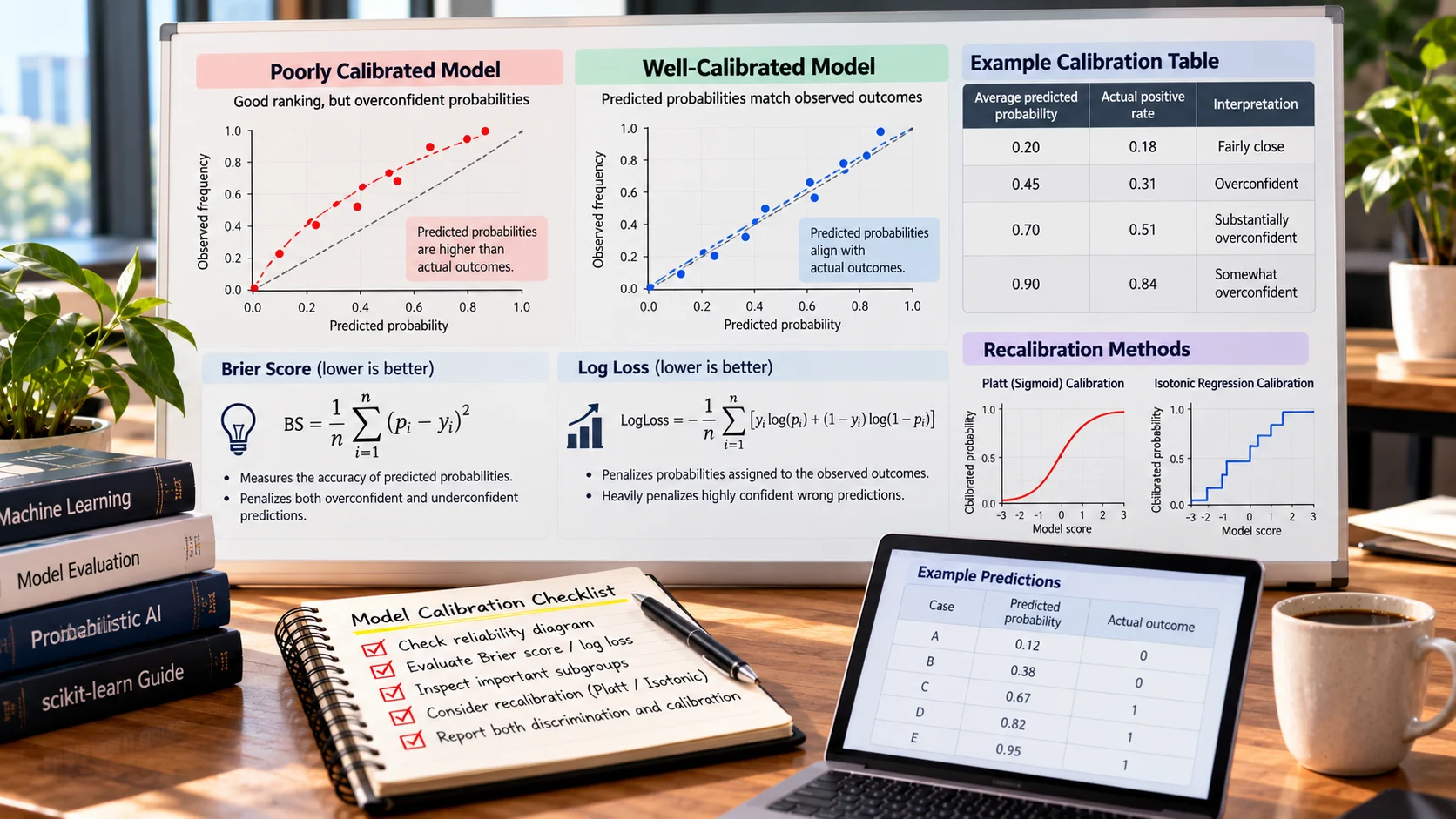
A reliability diagram groups predicted probabilities into bins and compares each bin’s average prediction with its observed outcome frequency. For example, among predictions around 0.7, did approximately 70% of the events happen? Ideally the points lie near the diagonal line where predicted probability equals observed frequency.
Consider an illustrative dataset with several buckets:
Average predicted probability Actual positive rate Interpretation
0.20 0.18 Fairly close
0.45 0.31 Overconfident
0.70 0.51 Substantially overconfident
0.90 0.84 Somewhat overconfident
These numbers are hypothetical, not an empirical evaluation of a named model. A reliability plot needs uncertainty intervals and an adequate number of observations in each bucket. Ten events in a bin cannot support the same confidence as ten thousand. Grouping choices also affect what the curve appears to show, so one chart should not be mistaken for a complete audit.
Calibration is about populations, not personal certainty
Suppose an insurer gives one claim a 60% probability of requiring further investigation. The claim will ultimately either require investigation or not. Calibration does not promise a 60%-correct partial outcome for that one case. It means that, among relevant cases with similar predicted scores, the observed frequency should be reasonably close to 60% under the evaluation conditions.
There can be many useful definitions of “relevant cases.” A classifier may be calibrated overall but misleading for a specific product, age group, geographic region, or season. For consequential uses, inspect meaningful segments and ensure there are enough observations for reliable comparisons. Protect privacy and avoid unjustified discriminatory uses when creating these groups.
Calibration is also conditional on the target and data distribution. A model calibrated for one country’s consumers or one company’s fraud patterns may not remain calibrated elsewhere. Changing base rates can distort the relationship between scores and outcomes even when ranking quality remains acceptable.
The Brier score and log loss
Calibration analysis often uses proper scoring rules. The Brier score for a binary event averages squared differences between predicted probability and observed outcome (zero or one). If a model predicts 0.8 and the event occurs, that one observation contributes (0.8 – 1)^2 = 0.04. If the event does not occur, it contributes (0.8 – 0)^2 = 0.64.
Log loss, also called cross-entropy loss in this context, penalizes probabilities assigned to observed outcomes and particularly punishes highly confident wrong predictions. Both metrics evaluate probability forecasts in ways that simple accuracy does not. However, neither is purely a measure of calibration: their values also reflect discriminatory ability and the inherent uncertainty of the problem.
This nuance is noted in scikit-learn’s calibration documentation. Teams should report complementary evidence: discrimination, calibration curves, proper scoring rules, subgroup behavior, and the costs of decisions made from the scores. A single “calibration score” cannot answer all of those questions.
How recalibration works
A calibration method learns a mapping from a model’s raw scores or predicted probabilities to better-aligned probabilities. Platt-style sigmoid calibration fits a sigmoid mapping, commonly suitable when the miscalibration pattern resembles that shape. Isotonic regression learns a nondecreasing mapping with fewer shape assumptions, but it can overfit when calibration data is scarce. Temperature scaling is a relatively simple method often used with neural-network logits; it changes their sharpness without generally changing the highest-ranked class.
No method creates information that was never present in the model’s score. Recalibration cannot repair systematic feature leakage, a fundamentally poor ranker, or severe shifts in who receives predictions. It may make the numbers more honest for the calibration population, but performance must be tested on fresh data.
Importantly, the calibrator should not be fit on the same observations used to train the underlying model without safeguards. Training predictions can appear unrealistically good; calibrating to them may create another optimistic result. Use independent calibration data or an appropriate cross-validation approach.
A safe experimental workflow
Start with a clear target definition: for example, probability that an order will be returned within 30 days of checkout. Next divide data into training, calibration, and final evaluation sets with boundaries appropriate to customers and time. Fit the base model on training data. Obtain scores on calibration data, fit the calibration mapping, and then evaluate both the original and calibrated predictions on the untouched evaluation set.
For recurring model updates, incorporate calibration checks into the release process. A new model architecture or class balance can change probability behavior even if overall accuracy improves. Do not select the method that best flatters the final holdout; use validation to choose among methods and preserve a realistic last test.
For live systems, record the model and calibrator versions together. If the base model changes while the calibrator remains old, the mapping may no longer be appropriate. Version them as one release artifact so rollback and audit procedures can reproduce the actual probability shown to users.
Python example with scikit-learn
This demonstration uses cross-validated calibration on an ordinary classification task. Substitute a chronology- or group-aware scheme if the deployment problem requires one.
from sklearn.calibration import CalibratedClassifierCV
from sklearn.linear_model import LogisticRegression
from sklearn.model_selection import train_test_split
from sklearn.metrics import brier_score_loss
X_train, X_test, y_train, y_test = train_test_split(
X, y, test_size=0.25, random_state=42, stratify=y
)
calibrated = CalibratedClassifierCV(
estimator=LogisticRegression(max_iter=1000),
method=”sigmoid”,
cv=5,
)
calibrated.fit(X_train, y_train)
probabilities = calibrated.predict_proba(X_test)[:, 1]
print(brier_score_loss(y_test, probabilities))
Check the installed scikit-learn version and adapt preprocessing to your data. This code does not replace reliability diagrams, subgroup testing, or a realistic deployment split. Nor does a low Brier score alone prove that probabilities are appropriate for every customer segment.
Choosing thresholds after calibration
A well-calibrated 70% probability does not tell a business whether an action is worthwhile. Thresholds depend on benefits, costs, capacity, and external obligations. A fraud-review team may tolerate more false alarms when potential losses are high. A customer-success team with limited staff may only contact a small group, prioritizing expected benefit rather than an arbitrary universal threshold.
For a simple hypothetical decision, suppose a successful intervention avoids an expected $100 loss, costs $12, and succeeds in 40% of cases that would otherwise have had the loss. Under oversimplified assumptions, the expected avoided loss is probability × 0.40 × $100. An action breaks even when this exceeds $12, giving a probability threshold of 0.30. Real decisions require better causal evidence and uncertainty estimates, but the example shows why calibrated probabilities are useful: they connect model outputs to expected value rather than only labels.
A predicted probability also should not be treated as a causal statement. High churn risk does not prove that sending a discount will prevent churn. Evaluate interventions separately with appropriate experimentation when possible.
Monitoring calibration after deployment
Monitor the delay before labels become available. In fraud detection, confirmed outcomes may arrive weeks later. In credit decisions, outcomes may take months. Evaluating only promptly labeled cases can introduce selection bias. Establish an outcome maturation window and track which records are still unresolved.
Compare reliability curves and proper scoring rules over time, both overall and in meaningful groups. Sudden changes in the positive-event base rate, scoring population, product mix, or upstream data definitions can make calibration stale. Use sufficient samples to avoid reacting to statistical noise. If recalibration is necessary, document why, retain independent evaluation, and check whether the underlying model itself should be retrained.
Our overview of AI benchmarks explains why a benchmark score does not fully determine operational suitability. Similarly, the guide to model parameters helps distinguish learned model behavior from the interpretation of reported output probabilities.
Frequent interpretation errors
A model that reports “confidence: 95%” may not output a statistically calibrated event probability at all. Generative assistants, for example, can produce fluent confidence phrases without a verified probability model behind them. Application designers should label such outputs carefully instead of letting prose imply quantified certainty.
Another common mistake is assessing only cases with known outcomes and ignoring unresolved or manually reviewed samples. This can bias calibration estimates. A third is comparing calibration across periods without accounting for changed outcome definitions. If one team treats cancellations as churn and another excludes them, the reliability curves measure different targets.
Finally, do not assume that improving calibration improves every metric. A monotonic mapping can preserve ranking while changing numeric probabilities; the gain is better correspondence between score and outcome frequency, not automatically a higher classification accuracy.
Calibration under changing class prevalence
Consider a fraud model trained when 1% of transactions were fraudulent. After a major product expansion, the fraud rate changes, or the types of attacks become different. Even if the model still ranks suspicious cases above ordinary ones, its probability mapping may no longer describe observed frequencies. A monitoring program should therefore watch the event rate, the composition of the scored population, and the reliability curve—not merely discrimination metrics.
Recalibration may be appropriate when the relationship between model scores and outcomes has shifted but meaningful ranking remains. Retraining may be necessary when important predictors change or the model can no longer separate cases. Neither decision should be made from one week of small-sample noise. Use sufficient observation windows and outcome maturation before changing production probabilities.
Why thresholds must be owned by the business
Suppose a predicted risk score is technically well calibrated, but the cost of one false alarm falls on a customer who is repeatedly denied service. The decision threshold is now an operational and ethical choice, not just a mathematical optimum. Teams should evaluate false-positive and false-negative consequences, customer appeal routes, fairness concerns, and resource capacity.
Document the threshold, business owner, approval date, and evidence used to set it. When a model is recalibrated, review the threshold again because an unchanged numerical cutoff may select a different set of cases. Record that change as part of the release—not as an invisible configuration detail.
How to interpret confidence in a small dataset
A calibration chart made from very few observations can look convincing without being stable. If a prediction bin contains just ten cases, one different outcome changes its observed success rate by ten percentage points. A smoother curve does not solve that sampling limitation automatically. Before trusting an apparently well-calibrated model, report how many examples contributed to each region, whether confidence intervals would be wide, and whether the same pattern appears on later data. Compare calibration separately for important subgroups when decisions affect them differently. A system can look calibrated overall while regularly overstating confidence for a smaller population. These checks are especially important when the score determines whether a human is asked to review a case, since a poorly calibrated threshold can quietly shift real work onto the wrong queue.
Reporting calibrated risk to nontechnical users
A forecast should communicate its target and time window, not just a naked percentage. “Estimated chance of a return within 30 days of purchase” is more informative than “80% confidence.” Where possible, provide an understandable uncertainty statement and explain when outcomes become measurable. In a dashboard, distinguish calibrated risk probability from a model’s raw classification score. Managers should know whether the number can reasonably support expected-cost calculations or should be used only to rank cases for further review.
When communicating to customers, avoid presenting a model probability as proof of wrongdoing or an individualized truth. Provide a process to correct underlying data and challenge consequential decisions. Clarity about what a score represents is part of responsible deployment.
Frequently asked questions
Is a 90% score always well calibrated if nine of ten events occur?
Ten observations are too few to establish reliable calibration. Larger representative samples, uncertainty assessment, and multiple probability regions are needed.
Can a model be calibrated but inaccurate?
Yes. Predicting a base rate near 10% for everyone can be calibrated when approximately 10% of cases are positive, but it may distinguish high-risk from low-risk cases poorly.
Does calibration remove bias?
No. Overall calibration does not guarantee equitable treatment or similar errors across groups. Calibration and fairness assessments address overlapping but distinct questions.
Conclusion
AI model calibration asks whether predicted probabilities deserve their numerical interpretation. Separate ranking from probability quality, evaluate on independent representative data, and use calibrated scores for decisions only after connecting them to actual costs and outcomes. Treat probabilities as measured forecasts with limitations, not as declarations of certainty.
References
scikit-learn: Probability calibration
scikit-learn: CalibratedClassifierCV