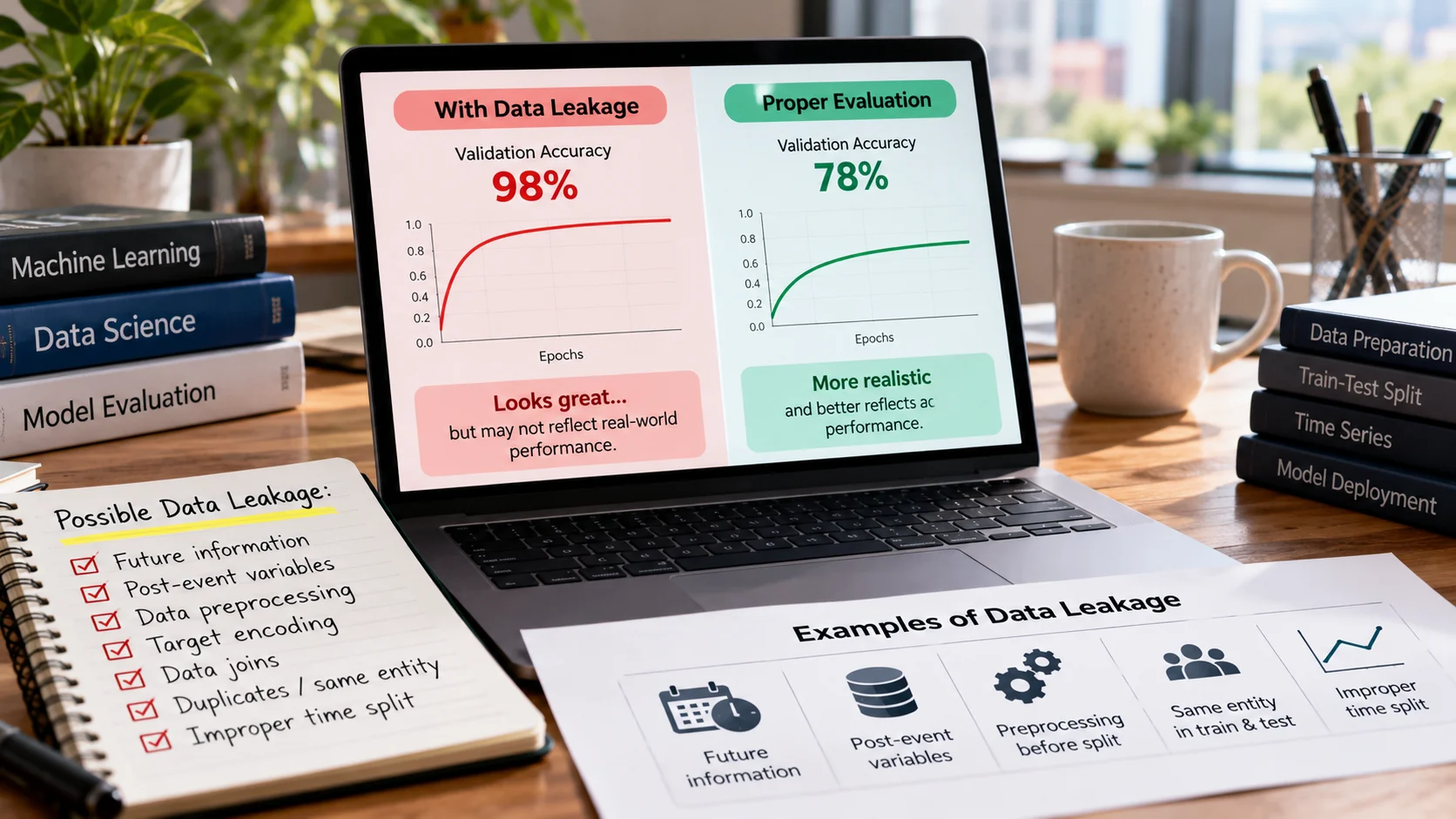
A machine-learning model can appear remarkably accurate in testing and disappoint as soon as it meets real customers. Sometimes the model was poorly designed. Sometimes the data changed. A more subtle explanation is AI data leakage: information reached training or evaluation that would not legitimately have been available when the prediction was made. The reported performance is then measuring a privileged experiment rather than the decision the business actually needs.
Leakage is especially dangerous because it can look like progress. A team adds a feature, validation accuracy rises, and the result seems convincing. Only later does somebody notice that the feature was generated after the event being predicted. Avoiding this mistake requires more than removing a suspicious column. It means designing the entire experiment around what was knowable at a precise moment in time.
Key takeaways
Data leakage occurs when a model or its evaluation uses information unavailable in the real prediction setting.
Leakage can enter through features, preprocessing, duplicate records, target encoding, data joins, time splits, or repeated model selection.
A random split is not always realistic for customers, patients, machines, or events that evolve over time.
The practical defense is to define a prediction timestamp, maintain train-only transformations, and test on truly independent cases.
What counts as leakage?
Imagine a retailer predicting whether an order will be returned. At checkout, it knows the customer, item category, delivery address, price, and previous purchasing history. The return authorization number, refund approval, and warehouse inspection report arrive later. If the training table includes the authorization number, a model may easily identify returned orders. The feature will not exist when the retailer wants to make its prediction, so the observed score is misleading.
This example is called target leakage: a feature contains information that directly or indirectly reveals the outcome. Other forms are less obvious. A marketing model can use a campaign response metric calculated after the campaign ended. An equipment model can include repair codes entered after a breakdown. A loan model can use an account status that is updated after the credit decision. In every case, the most useful diagnostic question is not whether the column is statistically predictive. It is when and how that value became available.
Data leakage is not the same as an ordinary, legitimate relationship between variables. A previous customer’s purchase history can reasonably predict future purchases if the history was available at the decision timestamp. A timestamped field that was backfilled next month cannot. The validity of a feature depends on the use case, not just its name or correlation.
Three common paths into a misleading model
Features that reveal the future
Predicting Friday’s sales using a Sunday inventory adjustment is a time-travel error even if the inventory adjustment sits in the same week’s reporting table. Business databases often record the latest value of a field rather than the value known at an earlier date. A retrospective join can therefore attach future knowledge to historical rows. Correct analysis may require event logs, historical snapshots, or a database capable of querying a record as of a point in time.
The risk grows when data teams join separate systems. A customer support table might use the case closing date to summarize a complaint, while the sales table represents information at the time the complaint began. Without explicit temporal rules, the final training set silently combines two different moments.
Train-test contamination
A model should not learn from its test set. Yet contamination can occur without placing the target labels in training. Suppose analysts standardize numeric features using the mean of the entire dataset before splitting. The test records have influenced the transformation. Similarly, selecting the ten strongest predictors using all available labels before splitting exposes the model-selection process to the test outcomes.
The correct order is to split first and learn preprocessing parameters only from training records. Apply those learned parameters to validation and test records without refitting. Libraries such as scikit-learn provide pipelines to enforce this separation; its official guide treats data leakage as a central modeling pitfall. A pipeline does not eliminate every risk, but it removes several common opportunities for accidental mixing.
Entities and duplicates crossing partitions
Two rows can be technically different while referring to the same underlying event. An image dataset may include different crops of one photograph. A medical dataset may include several visits from one patient. A help-desk dataset may include variations of the same conversation. If these related records appear on opposite sides of a random split, the test set is not truly unfamiliar.
Group-wise splitting can keep records from one patient, household, device, customer, or document family together. The appropriate group is determined by the intended deployment task: predicting a new visit for a known patient is different from generalizing to an entirely new patient. Both can be reasonable objectives, but they require different test designs.
Why ordinary cross-validation sometimes fails
Random cross-validation assumes that rows are sufficiently independent and that the future resembles the shuffled past. Those assumptions break down in chronological forecasting and some customer-level problems. If a model uses December records to help predict August, it may exploit seasonal or behavioral patterns that would not yet have been visible in August.
For a forecasting system, use forward-looking validation: train on January through June, validate on July; then train on January through July and validate on August. If the prediction involves events whose labels are revealed later, allow a gap between training and evaluation so delayed outcomes cannot cross the boundary. For grouped populations, apply a group-aware splitter rather than treating observations as independent. For data from several organizations, sometimes the most informative test is a previously unseen organization.
A practical validation plan specifies the data cutoff, eligible input features, label maturation window, and evaluation population. It also documents what happens when records are revised or deleted. This may seem slower than using a convenient random split, but it is faster than launching a model whose headline metric was never achievable in production.
Worked example: return prediction at checkout
Consider a simplified demonstration with 20,000 historical orders. The team builds two test designs. The first randomly divides the completed-order database and includes a field called refund_started. The model achieves an illustrative 96% classification accuracy. The second excludes all post-checkout fields and evaluates on the next calendar month’s orders. Its illustrative accuracy drops to 78%.
The difference does not prove that the second model is poor. It suggests that the first measurement was answering an easier question: identifying already-known returns rather than predicting future returns. To assess business usefulness, the team should also review precision and recall for the return class, false-positive handling costs, calibration, and stability by customer group. Overall accuracy can conceal weak performance when most orders are never returned.
A small point-in-time feature contract can prevent repeated errors:
Field Available at checkout? Use in model?
Item price at payment Yes Usually yes
Prior returns before payment Yes Yes, with proper history cutoff
Courier delivery exception recorded three days later No No
Refund request submitted after delivery No No
Delivery destination at checkout Yes Evaluate privacy and fairness implications
This table is a hypothetical example, not a result from a production model. Its purpose is to show how availability, not predictive strength alone, decides feature eligibility.
How to audit an existing dataset
First write the prediction statement in plain language: “At the moment an order is placed, estimate the chance of a return within 30 days.” Mark the exact timestamp and outcome window. Second, create a column-level inventory with source system, generation time, modification behavior, owner, and known missingness. Ask which features are retrospectively recalculated and whether their historical values can be reconstructed.
Third, trace every join. A join key may be correct while the joined row is from the wrong time. Use conditions such as event_time <= prediction_time where appropriate, and consider late-arriving data separately. Fourth, inspect the preprocessing code to ensure sampling, imputation, scaling, encoding, feature selection, and resampling all happen within training folds. Fifth, search for near-duplicates and overlapping entities. Sixth, compare results across random, time-based, and grouped splits, documenting why they differ rather than simply selecting the highest score. Finally, run an availability simulation. For several historical examples, attempt to reconstruct exactly what a live system would have seen at the decision moment. If the team cannot obtain a feature through the normal production workflow, do not include it merely because it makes the offline score better. Store these rules with the dataset contract, not in one analyst's memory. A leakage-aware scikit-learn pattern The following minimal pattern shows one useful safeguard: fitting preprocessing within a training pipeline after the split. Real applications must also handle chronological availability and grouping where relevant. from sklearn.model_selection import train_test_split from sklearn.pipeline import make_pipeline from sklearn.impute import SimpleImputer from sklearn.preprocessing import StandardScaler from sklearn.linear_model import LogisticRegression X_train, X_test, y_train, y_test = train_test_split( features, labels, test_size=0.2, random_state=42, stratify=labels ) model = make_pipeline( SimpleImputer(strategy="median"), StandardScaler(), LogisticRegression(max_iter=1000), ) model.fit(X_train, y_train) print(model.score(X_test, y_test)) This example assumes numeric features, reasonably independent records, and a valid split. It is not a drop-in recipe for time-series or grouped data. The benefit is that the imputer and scaler learn their parameters from training data during fit, rather than from the full dataset before partitioning. Signals worth investigating, not automatic proof A suspiciously high score is a prompt to investigate, not a mathematical definition of leakage. Some problems are genuinely easy. More useful warnings include one feature dominating the result without a plausible mechanism, a large drop from random-split accuracy to future-period accuracy, missing features at serving time, or model performance that collapses when late-arriving columns are removed. Also investigate unusually stable validation across changing business conditions and strong performance on customers represented in the training set but poor performance on new customers. An audit should identify the information path causing the problem. Simply deleting the best predictor can remove a legitimate feature while leaving actual leakage elsewhere. Model monitoring still matters after a clean evaluation. A model can pass leakage checks yet become less accurate when customer behavior changes after deployment. Fair comparisons between models depend on a well-defined test, which ByteScope discusses in its guide to AI evaluation benchmarks. Its explanation of how AI training data works adds context on data collection and model development. Leakage prevention and ongoing drift monitoring solve connected but distinct problems. Preventing leakage through team practices Make feature availability an acceptance criterion before model development begins. Data engineering should retain timestamped source records or controlled snapshots; modeling should document validation boundaries; product owners should clarify when decisions are made; and reviewers should test that the offline feature pipeline can be reproduced online. In regulated or consequential applications, retain the documentation needed to explain and reproduce these decisions. A review checklist can ask: What is the prediction time? When is the ground truth confirmed? Is every feature available then? Do rows overlap across partitions? Does any transformation fit on evaluation data? Have we repeatedly tuned against the nominal test set? Can the same feature be retrieved reliably in production? An independent reviewer should be able to answer these questions without relying on a model author's assurances. A release report that cannot hide the evaluation boundary A convincing model report should state more than the best score. Include the prediction timestamp, eligible input window, target definition, cutoff dates, entity grouping rules, feature generation versions, and the number of independent subjects in each partition. Where delayed outcomes are involved, explain when a label becomes final and how unresolved cases were treated. These details let a future reviewer reconstruct the conditions under which the prediction would have been made. Suppose an order-return model is trained on January–June orders and evaluated on July. If the return window is 30 days, the July labels may not mature until late August. Evaluating on July 31 and classifying still-open returns as negatives would introduce another misleading result. A correct release report records the maturation date and any excluded observations, even when that delays the presentation of results. Track deployment data availability as a separate gate. A feature can be leakage-free in historical evaluation and still fail operationally if the serving system retrieves it too slowly or occasionally returns a newer, backfilled value. Test offline and online feature parity using the same cutoff semantics. Accuracy matters only after the system can reproduce the experiment's information boundary in real time. Frequently asked questions Is data leakage the same as overfitting? No. Overfitting means a model learns details of its training sample that do not generalize well. Leakage means information crosses an invalid boundary in the data or evaluation process. Leakage can produce extremely flattering metrics even for relatively simple models. The two problems can coexist, but they need different investigations. Does a pipeline guarantee that a model is leakage-free? No. A correctly built pipeline helps isolate preprocessing, but it cannot tell whether an input column describes a future event, whether the dataset contains duplicates, or whether a training label was generated inappropriately. Domain knowledge and point-in-time data checks remain essential. Can test data ever be used during development? A validation set is used for iteration and model selection. A final holdout should remain independent for an unbiased last assessment. Once a holdout has repeatedly informed architecture or threshold choices, it effectively becomes another validation set; establish a fresh evaluation method rather than treating it as untouched. Bottom line The strongest leakage defense is to reconstruct the actual decision your model will make: for whom, at what time, with which information. Split the data to reflect that setting, fit preprocessing only where permitted, and interrogate unusually good results. A slightly lower but realistic estimate of model quality is much more valuable than an impressive score that cannot survive contact with production. References scikit-learn: Common pitfalls and recommended practices scikit-learn: Pipeline user guide